Functional analysis

Functional analysis is the process of taking a list of genes which we cannot meaningfully interact with and distilling information that we as researchers can then interpret. Generally, this involves grouping genes based on functions or processes, and determining which processes or functions appear to be different between your experimental groups.

There are different approaches to functional analysis e.g.,:

Over-representation analysis: are certain processes, pathways or biological functions over-represented in a list of differentially expressed genes relative to the background genome (often called Gene Ontology analysis).
Functional class scoring (Gene Set Enrichment Analysis (GSEA)): Rather than taking a list of differentially expressed genes (which are themselves based on thresholds and cutoffs defined by a user), GSEA takes the ranked position of all genes to see how pathways and processes are perturbed.
Pathway topology: Pathway topology analysis takes a higher level approach, compiling information on up- and down-regulation at the level of the pathway rather than the level of the gene.

Today we will cover Over-representation analysis and functional class scoring. Links to pathway topology workflows are provided.

Annotation

The basis of this stage of the analysis is to take individual genes, associate them with a function, and then to identify whether there are common themes of function in genes which have undergone changes in gene expression.

This first requires that our genes are annotated - we must be able to associate some type of function or process with a given gene. There are now many databases that maintain information and annotation on genes, including proposed and confirmed functions, pathways, processes etc.,. Annotation and databases is an entire area in itself, and not something we can cover today. For now, we will retrieve annotation information from different sources and attach the annotation to genes.

Over-representation Analysis

The hypergeometric distribution

Let’s say you have a list of 100 differentially expressed genes and, after annotation, you notice that 10 of these genes are involved in apoptosis. Is this a significant finding? Initially, you might think that yes it is significant, since 10% of your genes of interest share a role. However, to understand whether this is significant we need to consider the number of apoptosis-related genes in the genome. If, for example, we find that 12% of all genes in the genome are annotated as apoptosis-related, then seeing 10% of your differentially expressed genes with this annotation isn’t significant - it’s approximately what you would have expected. However, if you’d found 25% (or 0%!) THEN you might have something significant.

Over-representation analysis is the use of a hypergeometric distribution to determine whether or not a sample group is undergoing coordinated gene expression changes. Statistically, it is asking what is the probability of getting 10 apoptosis genes in my list of 100 differentially expressed genes, given the number of apoptosis genes in the whole genome. We can use the Fisher’s Exact test and the hypergeometric distribution to ask whether being involved in apoptosis is independent of being significantly differentially expressed.

What does this look like in practice? We can use a 2 x 2 table, where the four data points are (from top left to bottom right): the number of genes that are both in the category and are differentially expressed, the number of differentially expressed genes not in the category, the number of category genes that are not differentially expressed, and the number of genes that are neither in the category nor differentially expressed.

Let’s attach some real numbers to those categories and visualise them. We have 10 apoptosis genes in our 100 differentially expressed genes, there are 500 genes annotated as apoptosis, and a total of 10,000 genes in the genome.

hypergeoDistMatrix <- matrix(c(10,490,90,9410),2,2)
hypergeoDistMatrix

     [,1] [,2]
[1,]   10   90
[2,]  490 9410

Quickly, where did these numbers come from?

Top left: 10 differentially expressed genes which are apoptosis related.

Top right: 90 genes that are differentially expressed but are not apoptosis related.

Bottom left: 490 genes that are apoptosis related but not differentially expressed.

Bottom right: 9410 genes that are neither differentially expressed or apoptosis related.

Row 1 sums to 100 (differentially expressed genes)

Row 2 sums to 9,900 (non-differentially expressed genes)

Col 1 sums to 500 (apoptosis genes)

Col 2 sums to 9,500 (non-apoptosis genes)

Now we can test for an association - or, more accurately, we can test the null hypothesis that being in the apoptosis category is independent of being in the differentially expressed category.

fisher.test(hypergeoDistMatrix)


    Fisher's Exact Test for Count Data

data:  hypergeoDistMatrix
p-value = 0.03328
alternative hypothesis: true odds ratio is not equal to 1
95 percent confidence interval:
 0.9832142 4.1416491
sample estimates:
odds ratio 
  2.133664

The p-value of 0.033 let’s us reject the null hypothesis and we conclude there is an association. In our hypothetical experiment, apoptosis-related genes are over-represented (enriched) in our differentially expressed gene list.

We don’t want to perform this test manually for every possible functional category (adjusting for multiple testing as we go), so we will look to existing software packages to do this for us. But first, let’s look at some caveats and considerations.

Caveats

The hypergeometric distribution and Fisher’s test makes the assumption that all genes are equal. As an exercise, take 30 seconds to think about the ways that genes might not be equal, about RNA-sequencing, and what impact this could have on our test.

One major difference when looking across genes is gene length. RNA-seq tends to produce greater counts for longer genes, which is itself worth remembering, and this gives these genes a greater chance of being statistically differentially expressed. An additional problem is that some gene sets tend to be made up of primarily long genes (because certain processes or functions may require large, complex proteins). Because long genes have a greater chance of being differentially expressed, gene sets which are made up of long genes will have a greater chance of being enriched or over-represented.

We must carry out some type of correction for gene length when conducting over-representation analyses.

GOseq

We will begin with a method called GOseq, which was developed as part of one of the publications initially identifying the gene length bias. An illustration from the full paper is below, demonstrating the relationship between differential gene expression and gene length and between differential expression and number of reads. 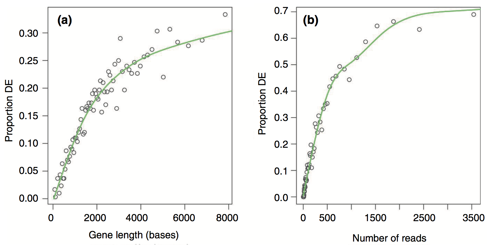Young et al., (2010) demonstrates bias due to gene length and expression

There is a strong positive correlation between differential gene expression and both total gene length and number of reads. Unless corrected for, gene length will bias your over-representation analysis.

Load the goseq package, the dplyr package (if you haven’t already), and use the supportedOrganisms() function to check whether your organism of interest is supported. The code for Saccharomyces cerevisiae is sacCer.

library(dplyr)


Attaching package: 'dplyr'

The following objects are masked from 'package:stats':

    filter, lag

The following objects are masked from 'package:base':

    intersect, setdiff, setequal, union

library(goseq)

Loading required package: BiasedUrn

Loading required package: geneLenDataBase

supportedOrganisms() %>% View()

We need to create an object that will pass GOseq a list of all our genes, with the differentially expressed genes highlighted. To do this, we will use an ifelse() statement which will check every gene in our experiment and ask test if it has an adjusted p-value of less than 0.05. If adj-p-value is < 0.05, return a “1” and if greater than (or equal to) 0.05, return a “0”. After that, add the gene names to this vector of 1s and 0s.

Note #1: at the end of the previous exercise we also applied a logFC threshold for defining differentially expressed. We won’t use that here and will just use adjusted p-values for simplicity.

Note #2: the tt object was created when we used limma to identify differentially expressed genes. tt is 7,127 rows, and has genes stored as row names, includes the logFC, and adj.P.Val columns.

load("tt.RData")

genes <- ifelse(tt$adj.P.Val <= 0.05, 1, 0)

names(genes) <- rownames(tt)

head(genes)

YAL038W YOR161C YML128C YMR105C YHL021C YDR516C 
      1       1       1       1       1       1

tail(genes)

YOR122C YJR139C YEL046C YDL084W YOR326W YOL120C 
      0       0       0       0       0       0

Note #3: because tt is ordered (that is, all the genes with low p values are at the top), it’s worth using tail to check the bottom of the new genes object looks different to the top. Another useful check is to use the table() function to ask how many genes fall into each category.

table(genes)

genes
   0    1 
1987 5140

This is a useful reminder about the conditions of this experiment: of the 7,127 genes in the tt object, 5,140 are differentially expressed. Most experiments will not have this level of differential expression.

IF you did want to include the logFC cutoff, you can use the code below. This gives a more modest 1,891 differentially expressed genes. For the purposes of today’s workflow, we will continue with the larger gene list.

genes2 <- ifelse(tt$adj.P.Val <= 0.05 & (abs(tt$logFC) > log2(2)), 1, 0)
names(genes2) <- rownames(tt)
table(genes2)

genes2
   0    1 
5236 1891

Methodology

What is GOSeq doing? How does it correct for gene length?

Remember that we will still use the hypergeometric distribution and Fisher’s Exact test with the 2 x 2 table. Because we know that longer genes are more likely to in the differentially expressed category, we can think of this category as having more weight than it should. GOSeq will calculate a value for each gene which will offset this artificial weight. In other words, if our 2 x 2 table would have 10 genes in the top left square, and some of those genes are very long, GOSeq will treat the number as something slightly less than 10. By treating the value as less than 10, we have taken into account the fact that there shouldn’t really have been 10 genes in there in the first place if not for gene length bias.

Calculate the weighting that should be assigned to each gene with the Probability Weighting Function (the nullp() function). Specify the object “gene” which is our list of all genes and whether they are differentially expressed or not, as well as the genome (“sacCer1” for our yeast genome), and the gene ID type. This will create a plot in which genes are placed into “bins” based on length, and then gene length vs proportion of differentially expressed is plotted. We can then inspect the pwf object.

pwf = nullp(genes, "sacCer1", "ensGene")

Loading sacCer1 length data...

Warning in pcls(G): initial point very close to some inequality constraints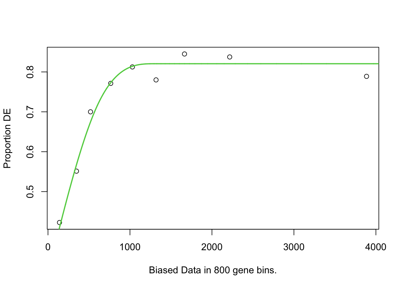

pwf %>% head()

        DEgenes bias.data       pwf
YAL038W       1      1504 0.8205505
YOR161C       1      1621 0.8205505
YML128C       1      1543 0.8205505
YMR105C       1      1711 0.8205505
YHL021C       1      1399 0.8205505
YDR516C       1      1504 0.8205505

pwf %>% tail()

        DEgenes bias.data       pwf
YOR122C       0       383 0.5916345
YJR139C       0      1081 0.8170373
YEL046C       0      1165 0.8196654
YDL084W       0      1342 0.8205505
YOR326W       0      4726 0.8205505
YOL120C       0       563 0.6975162

Here we can see that genes have been given a different pwf value based on the bias.data column. The pwf value will be less than 1, and indicates how much a gene should be ‘counted for’ if it is in the differentially expressed category in the 2 x 2 table.

We can predict that pwf and bias (length) are opposing values, and we can visualise that data:

par(mfrow=c(1,2))
hist(pwf$bias.data,30)
hist(pwf$pwf,30)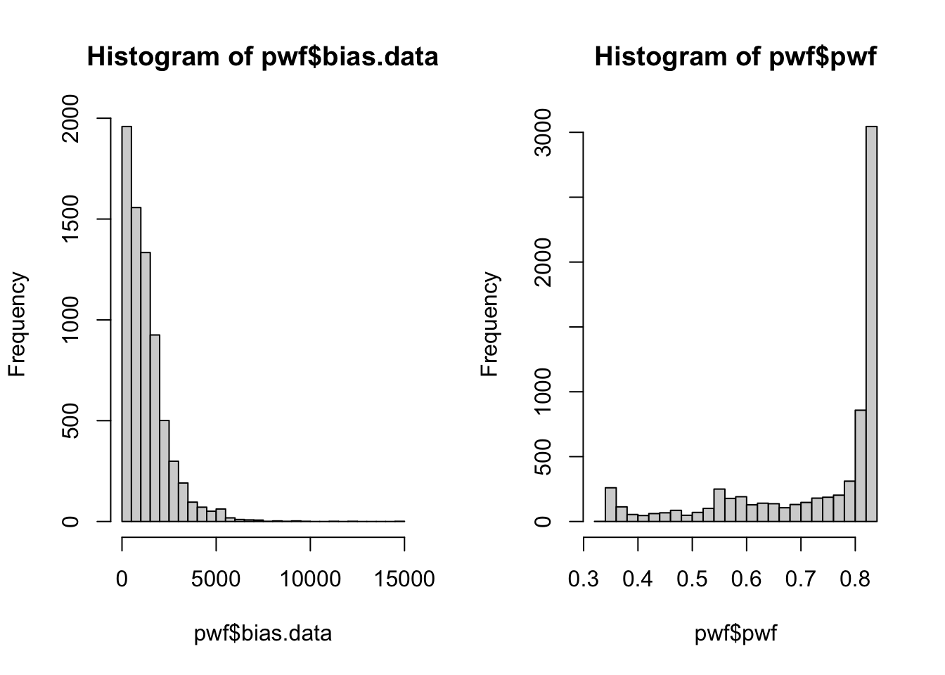

We have a large number of genes which have low/no bias, and a correspondingly high number of genes with the max pwf weighting. A smaller number of genes have a greater bias and are given lower weighting.

We can now carry out our Fishers Exact test using the pwf value instead of the raw counts. We will use the goseq() function to perform this test, and output the over-representation data into an object.

# BiocManager::install("org.Sc.sgd.db")
# BiocManager::install("AnnotationDbi")
library(org.Sc.sgd.db)

Loading required package: AnnotationDbi

Loading required package: Biobase

Welcome to Bioconductor

    Vignettes contain introductory material; view with
    'browseVignettes()'. To cite Bioconductor, see
    'citation("Biobase")', and for packages 'citation("pkgname")'.


Attaching package: 'AnnotationDbi'

The following object is masked from 'package:dplyr':

    select

GO.wall = goseq(pwf, "sacCer1", "ensGene")

Fetching GO annotations...

For 1325 genes, we could not find any categories. These genes will be excluded.

To force their use, please run with use_genes_without_cat=TRUE (see documentation).

This was the default behavior for version 1.15.1 and earlier.

Calculating the p-values...

'select()' returned 1:1 mapping between keys and columns

GO.wall %>% head()

       category over_represented_pvalue under_represented_pvalue numDEInCat
1239 GO:0005622            1.826445e-17                        1       4300
4848 GO:0042254            5.046546e-12                        1        369
3578 GO:0022613            2.239622e-11                        1        442
7249 GO:0110165            4.401672e-11                        1       4467
8128 GO:1990904            5.902761e-11                        1        469
5039 GO:0043228            9.417045e-11                        1       1266
     numInCat                                 term ontology
1239     5183   intracellular anatomical structure       CC
4848      400                  ribosome biogenesis       BP
3578      486 ribonucleoprotein complex biogenesis       BP
7249     5434           cellular anatomical entity       CC
8128      525            ribonucleoprotein complex       CC
5039     1464       non-membrane-bounded organelle       CC

We will want to filter for only those categories with an adjusted p-value < 0.05, and save that information to a new object for easy browsing.

You might have noticed that the GO.wall object doesn’t automatically perform an adjustment for multiple testing, so we will use the p.adjust() function to generate corrected p-values.

We will then use the adjusted p-values as a filtering criteria, and include the columns that correspond to category, term, and ontology (using the colnames() function, we can see that these are columns 1, 6 and 7).

GO.wall.padj = p.adjust(GO.wall$over_represented_pvalue, method="fdr")

sum(GO.wall.padj < 0.05)

[1] 49

GO.wall.sig = GO.wall[GO.wall.padj < 0.05, c(1,6,7)]

GO.wall.sig %>% dim()

[1] 49  3

GO.wall.sig %>% head()

       category                                 term ontology
1239 GO:0005622   intracellular anatomical structure       CC
4848 GO:0042254                  ribosome biogenesis       BP
3578 GO:0022613 ribonucleoprotein complex biogenesis       BP
7249 GO:0110165           cellular anatomical entity       CC
8128 GO:1990904            ribonucleoprotein complex       CC
5039 GO:0043228       non-membrane-bounded organelle       CC

An optional filtering step can be applied here, which is to remove categories that have a large number of genes. Categories which have a large number of genes tend to be very broad terms, which are not very informative e.g., the categories “organelle”, “biological_process”, and “protein localization”.

If you choose to apply this filter, re-make the GO.wall.sig object. Here we are filtering with a requirement that the category contains fewer than 500 genes.

GO.wall.sig <- GO.wall[GO.wall.padj < 0.05 & GO.wall$numInCat < 500, c(1,6,7)]

GO.wall.sig %>% dim()

[1] 20  3

GO.wall.sig %>% head()

       category                                 term ontology
4848 GO:0042254                  ribosome biogenesis       BP
3578 GO:0022613 ribonucleoprotein complex biogenesis       BP
3742 GO:0030684                          preribosome       CC
1600 GO:0006364                      rRNA processing       BP
4526 GO:0034470                     ncRNA processing       BP
2966 GO:0016072               rRNA metabolic process       BP

This is a very useful way of getting a broad overview of what processes our differentially expressed genes are involved in. The final step we will take here is to use the GO.db package to retrieve more detailed information about the categories we have identified. GO.db will use the unique identifier in the category column and provide more information.

library(GO.db)

GOTERM[[GO.wall.sig$category[1]]]

GOID: GO:0042254
Term: ribosome biogenesis
Ontology: BP
Definition: A cellular process that results in the biosynthesis of
    constituent macromolecules, assembly, and arrangement of
    constituent parts of ribosome subunits; includes transport to the
    sites of protein synthesis.
Synonym: GO:0007046
Synonym: ribosome biogenesis and assembly
Secondary: GO:0007046

Closing thoughts on GOseq

GOSeq is a powerful tool that corrects for an important bias in RNA-seq data. There are other options when it comes to over-representation analysis, and functional analysis in general. Some of these tools might help with generating better visualisations, or claim to have more up-to-date databases.

Gene set enrichment analysis and clusterProfiler

We will not complete a full demonstration of gene set enrichment analysis (GSEA) and clusterProfiler, but we will give an overview of these techniques and tools.

In particular we strongly recommend The Carpentries workshop RNA-sq analysis with Bioconductor section on GSEA.

GSEA

GSEA takes an alternative approach to the previous section in that it does not take as input a list of differentially expressed genes. GSEA moves away from the binary “differentially expressed or not” approach and considers the state, or position, of all genes in the list.

This approach has the advantage of not relying on our somewhat arbitrary cutoff thresholds (e.g., a gene with a p-value 0.0501 probably should still contribute to what we think is happening to a pathway).

ClusterProfiler

ClusterProfiler is a widely used package with the support to create excellent figures (check these out).

GSEA, clusterProfiler and length correction

GSEA and clusterProfiler do not implement a gene length correction. Does this invalidate them as options? We argue that it does not. Even without length correction, GSEA is implementing a powerful and logical approach and the visualisations made with clusterProfiler should not be under-valued.

In any situation where there are multiple tools, methods, or decision points (e.g., thresholds, removal of outliers etc.,) it is recommended that you complete the analyses and compare the outcomes. It is possible to run GOSeq without the length correction implemention (shown below) and compare the over-represented categories. If the difference is large, then you should be cautious when interpreting GSEA results or the output of clusterProfiler.

GO.nobias=goseq(pwf, "sacCer1", "ensGene", method="Hypergeometric")

Fetching GO annotations...

For 1325 genes, we could not find any categories. These genes will be excluded.

To force their use, please run with use_genes_without_cat=TRUE (see documentation).

This was the default behavior for version 1.15.1 and earlier.

Calculating the p-values...

'select()' returned 1:1 mapping between keys and columns